An application I work on has a reporting engine that uses Excel for report templates. When a report is generated, the code adds a "Data" worksheet to the Excel template, and populates it with named ranges of tabular data. User-defined template worksheets can then use formulas such as VLOOKUP and MATCH to reference and display values from the Data worksheet's named ranges.
For a particular template I needed to get the maximum value of a column of numbers in one of the Data worksheet's named ranges. The problem I ran into was that I didn't know at what row the named range would start, and how many rows it would have, because each time the Data worksheet generates, the various named ranges could have a different number of rows.
For a particular template I needed to get the maximum value of a column of numbers in one of the Data worksheet's named ranges. The problem I ran into was that I didn't know at what row the named range would start, and how many rows it would have, because each time the Data worksheet generates, the various named ranges could have a different number of rows.
The key to the solution I came up with was to use the INDIRECT Excel function. Here's Microsoft's definition of the function:
Returns the reference specified by a text string. References are immediately evaluated to display their contents. Use INDIRECT when you want to change the reference to a cell within a formula without changing the formula itself.
In other words, the INDIRECT function is way to "macro substitute" (a term for those of you as old-school as me), to dynamically evaluate a string reference expression.
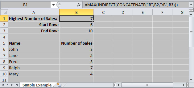
Figure 1 shows a simple example of using INDIRECT to get a MAX value from a range of column values:
Figure 1 shows a simple example of using INDIRECT to get a MAX value from a range of column values:
In the Figure 1 example, the starting and ending rows are known, so the INDIRECT isn't really needed. However, you can see in the function field that the INDIRECT is concatenating column letters with row numbers to create a reference. In this case the resulting reference is "B6:B10". That reference is then being passed to the MAX function, producing the correct value of seven.
But what if you didn't know what the column's start and end row numbers were going to be, but you did know that they'd be encompassed in a named range? That's what I was faced with. I knew the name of the named range that contained the values. I also knew what column the values would be in. What I did not know were the first and last row numbers of the range. The solution I found was the INDIRECT function. (If you know a better way, please comment!)
But what if you didn't know what the column's start and end row numbers were going to be, but you did know that they'd be encompassed in a named range? That's what I was faced with. I knew the name of the named range that contained the values. I also knew what column the values would be in. What I did not know were the first and last row numbers of the range. The solution I found was the INDIRECT function. (If you know a better way, please comment!)
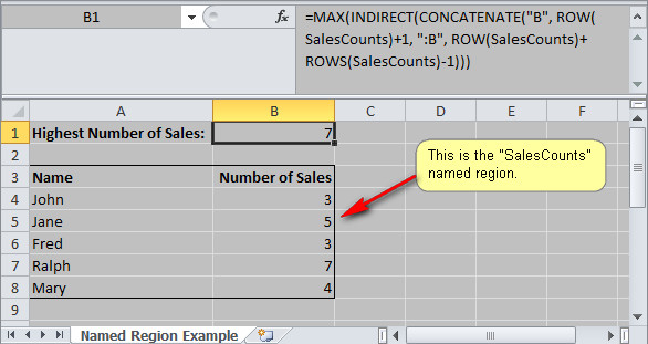
Figure 2 shows an example that uses ROW and ROWS to find the first and last row numbers of the range, which are then used in the INDIRECT function, which is used by the MAX function:
Here's the complete function, in text, if you want to copy it:
=MAX(INDIRECT(CONCATENATE("B", ROW(SalesCounts) + 1, ":B", ROW(SalesCounts) + ROWS(SalesCounts) - 1))) When determining the starting row, because the SalesCounts region includes the headers, 1 is added to the result of the ROW(SalesCounts) function call (3 + 1 = 4). When determining the ending row, the number of rows is determined using ROWS(SalesCounts), added to the starting row, and then 1 is subtracted (3 + 6 - 1 = 8).
If the named region you need to reference is on a different worksheet (for example, a worksheet named "Data"), simply include the name of the worksheet when concatenating the reference string, like this:
If the named region you need to reference is on a different worksheet (for example, a worksheet named "Data"), simply include the name of the worksheet when concatenating the reference string, like this:
=MAX(INDIRECT(CONCATENATE("Data!B", ROW(SalesCounts) + 1, ":B", ROW(SalesCounts) + ROWS(SalesCounts) - 1))) You could of course get a SUM of the column, instead of the MAX, or perform other functions using this same technique.
| Click on the link to the right to download an example Excel file. |
| ||


 RSS Feed